dbinom(c(1, 1, 0), size = 1, prob = -1)Warning in dbinom(c(1, 1, 0), size = 1, prob = -1): NaNs produced[1] NaN NaN NaNWhat’s the relationship between logit and likelihood?
What is the logit?
is Bernoulli(p) the same as logit(p)?
It’s a transformation!
Problem:
Given the equation
\[ y = \beta_0 + \beta_1 x \]
Depending on the values on the right hand side of the equation, y can be any real number.
In logistic regression, we’ll need to calculate the likelihood of some 0’s and 1’s given a probability \(p\). If our \(p\) is outside [0, 1] that’s undefined.
I can’t do this:
dbinom(c(1, 1, 0), size = 1, prob = -1)Warning in dbinom(c(1, 1, 0), size = 1, prob = -1): NaNs produced[1] NaN NaN NaNWhen we try to use probabilities outside [0,1] we get Not A Number.
That’s where the logit comes in.
\[ odds = \frac{p}{1-p} \\ logit = log(odds) \]
library(tidyverse)── Attaching core tidyverse packages ──────────────────────── tidyverse 2.0.0 ──
✔ dplyr 1.1.4 ✔ readr 2.1.5
✔ forcats 1.0.0 ✔ stringr 1.5.1
✔ ggplot2 3.5.0 ✔ tibble 3.2.1
✔ lubridate 1.9.3 ✔ tidyr 1.3.1
✔ purrr 1.0.2
── Conflicts ────────────────────────────────────────── tidyverse_conflicts() ──
✖ dplyr::filter() masks stats::filter()
✖ dplyr::lag() masks stats::lag()
ℹ Use the conflicted package (<http://conflicted.r-lib.org/>) to force all conflicts to become errorsp <- seq(0.01, 0.99, length.out = 100)
odds <- p / (1 - p)
logit <- log(odds)
tibble(p, odds, logit) %>%
ggplot(aes(p, odds)) +
geom_line()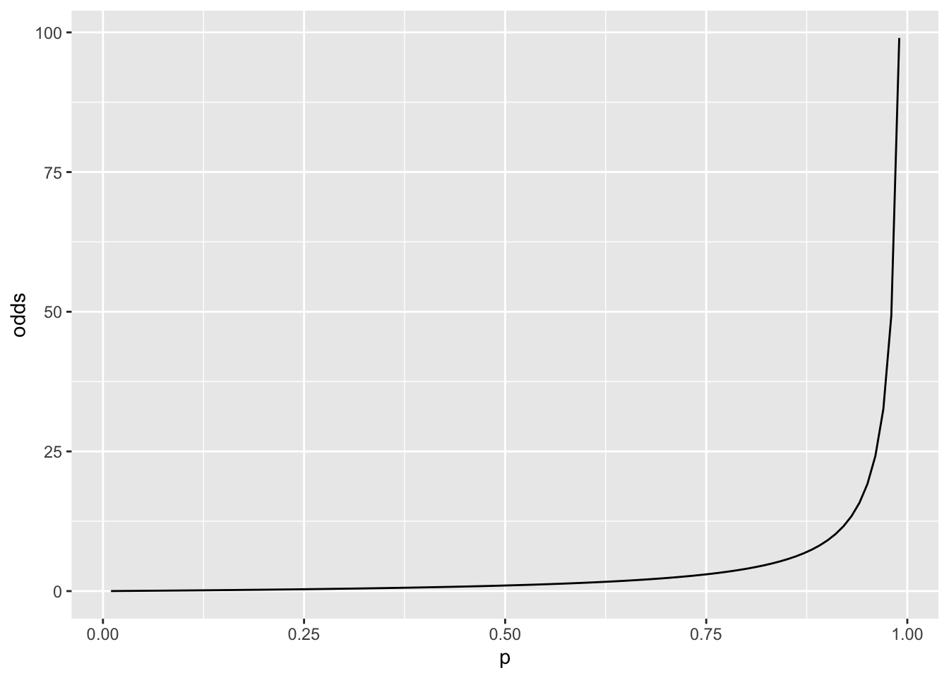
# When p = 0.5, odds = 1
# ditto,        logit = 0

tibble(p, odds, logit) %>%
  ggplot(aes(p, logit)) +
  geom_line()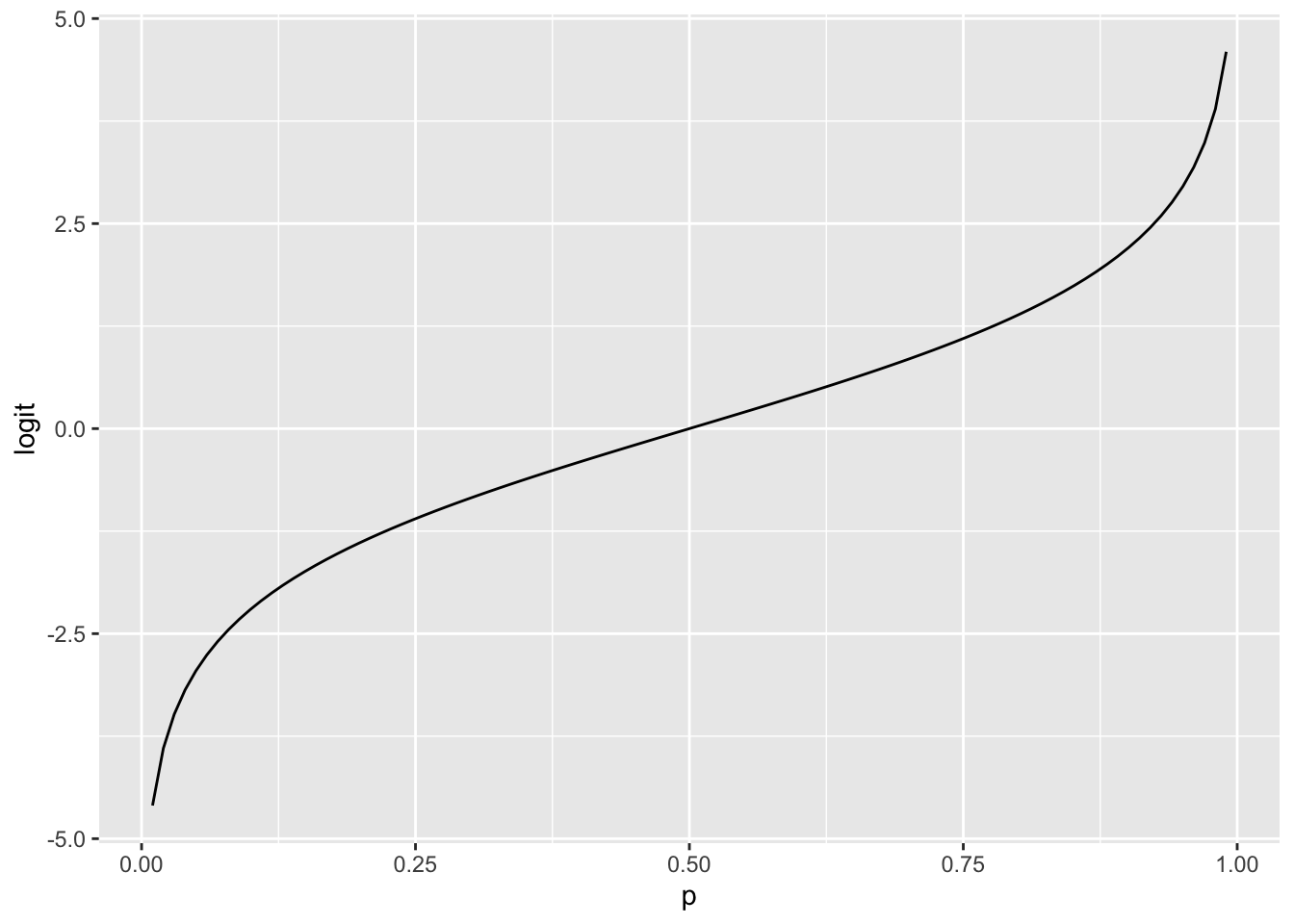
logit converts what we have (0, 1) to what we can model (-Inf, Inf)
Allows us to treat a probability as a linear model.
\[ \text{endangered} \sim Bernoulli(p) \\ logit(p) = \beta_0 + \beta_1 \text{dist2coast} \]
set.seed(1422)
# Step 1, generate predictors
dist2coast <- runif(100, 0, 100)
# Step 2, choose our coefficients
beta_0 <- 0
beta_1 <- -0.1
# Step 3, calculate random variable parameters (in this case, just p)
logit_p <- beta_0 + beta_1 * dist2coast
inv_logit <- function(x) exp(x) / (1 + exp(x))
p <- inv_logit(logit_p)
# Step 4, generate random numbers from the random variable
endangered <- rbinom(100, size = 1, prob = p)
# Done! Simulated!

# Let's visualize
tibble(dist2coast, p, endangered) %>%
  ggplot(aes(dist2coast)) +
  geom_point(aes(y = endangered)) +
  geom_line(aes(y = p), color = "firebrick") +
  theme_bw()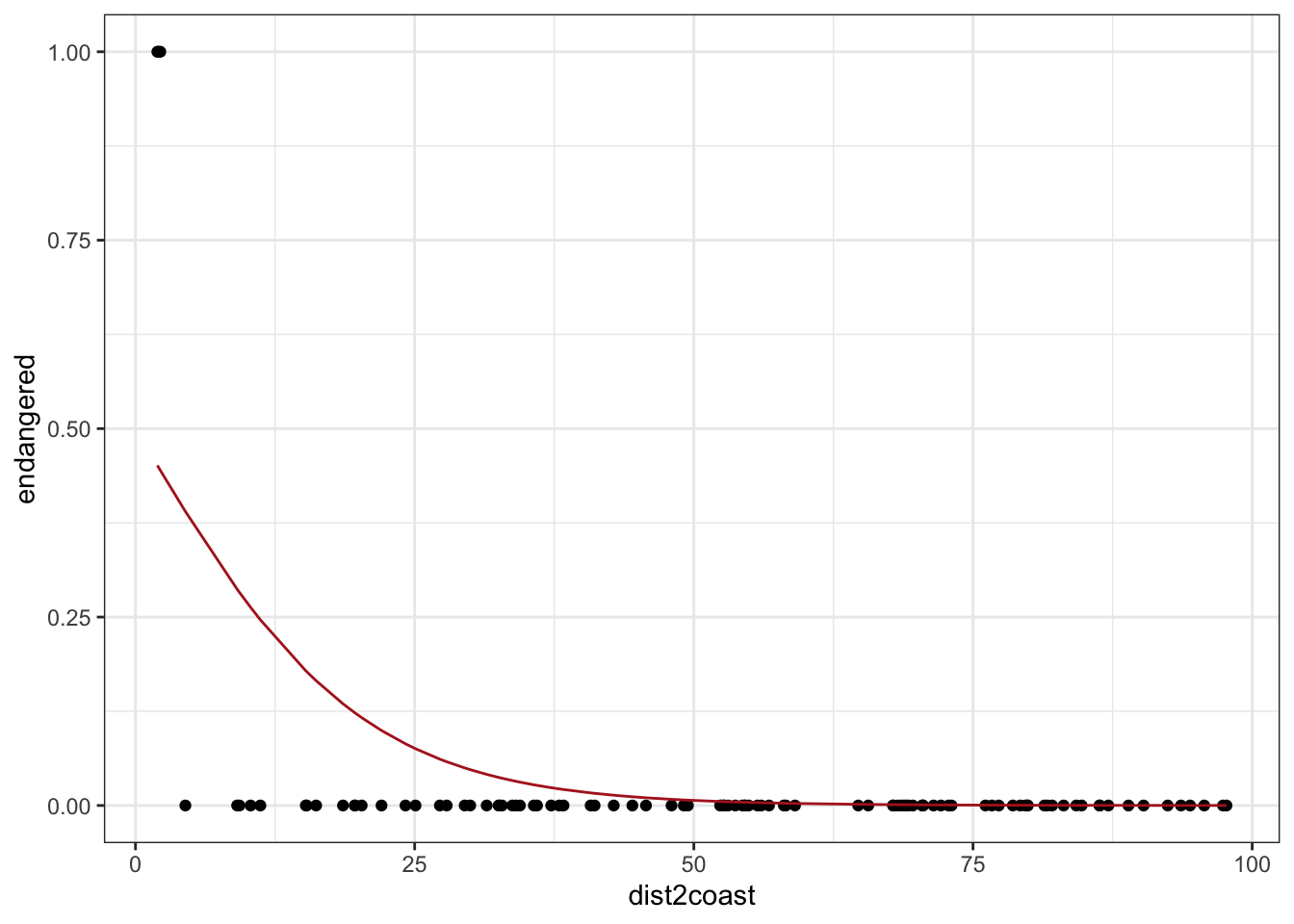
p declines as we move away from the coast (red line)
only “success” we saw was when p was closest to 1 (i.e. all the way to the left)
Now, how would I make the red line increase as we move away from the coast?
set.seed(1422)
# Step 1, generate predictors
dist2coast <- runif(100, 0, 100)
# Step 2, choose our coefficients
beta_0 <- -1
beta_1 <- 0.1
# Step 3, calculate random variable parameters (in this case, just p)
logit_p <- beta_0 + beta_1 * dist2coast
inv_logit <- function(x) exp(x) / (1 + exp(x))
p <- inv_logit(logit_p)
# Step 4, generate random numbers from the random variable
endangered <- rbinom(100, size = 1, prob = p)
# Done! Simulated!

# Let's visualize
tibble(dist2coast, p, endangered) %>%
  ggplot(aes(dist2coast)) +
  geom_point(aes(y = endangered)) +
  geom_line(aes(y = p), color = "firebrick") +
  theme_bw()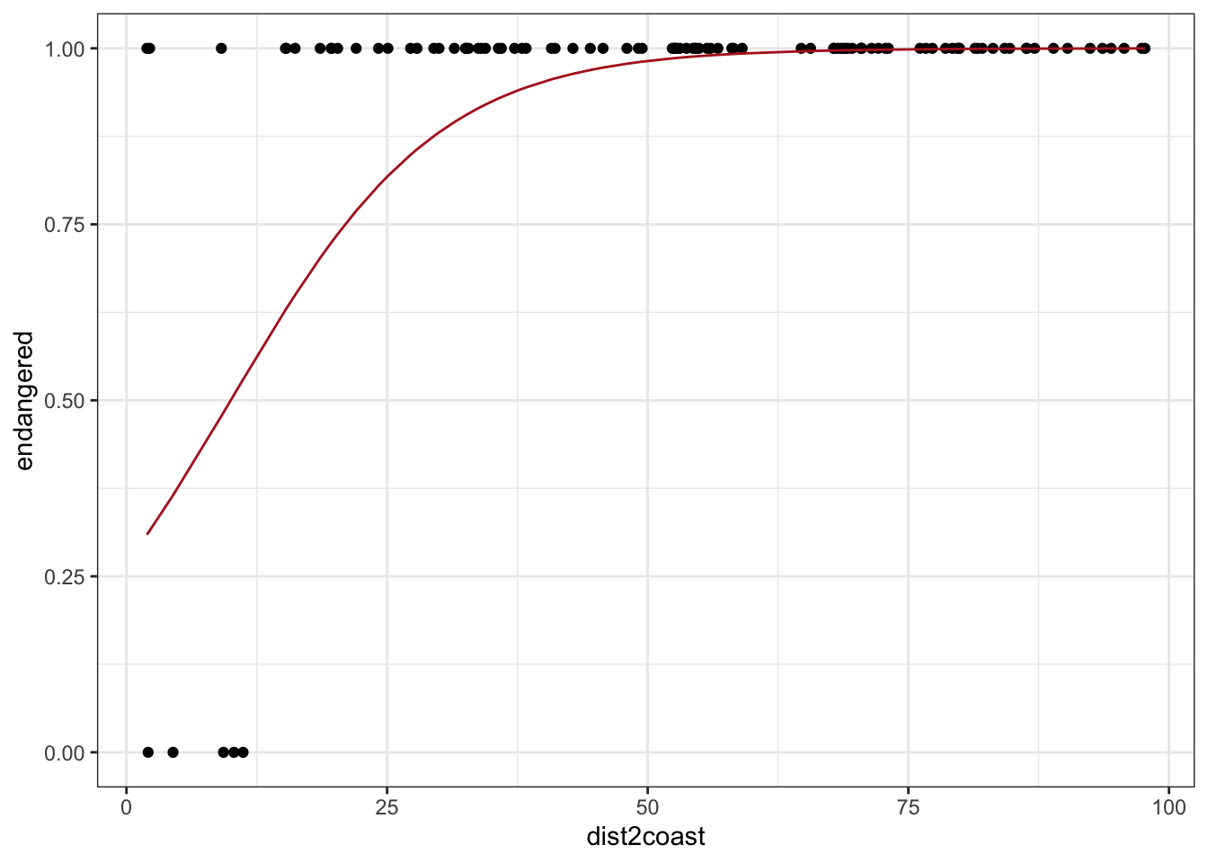
logit is a transformation. It’s a formula applied to an input.
\[ logit(x) = log(\frac{x}{1-x}) \]
Bernoulli is a random variable. “distributed as”
p <- 0.75
x <- 0:1
PMF_p <- c(1 - p, p)

tibble(p, PMF_p, x) %>%
  ggplot() +
  geom_segment(aes(x = x, xend = x, y = 0, yend = PMF_p)) +
  geom_point(aes(x, PMF_p), size = 2) +
  expand_limits(y = 1) +
theme_bw() 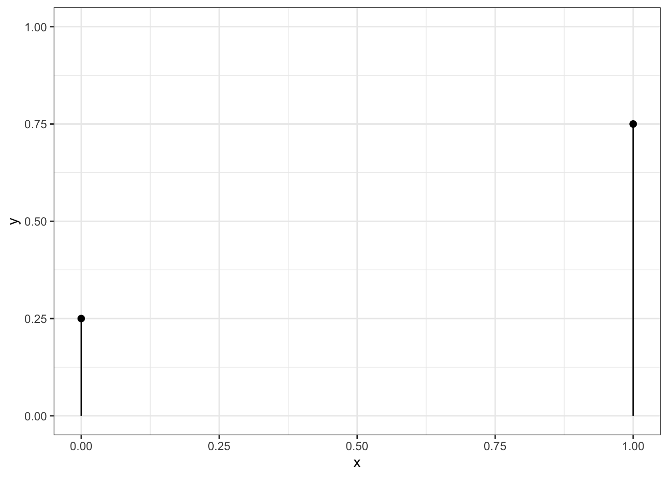
What’s the likelihood of p being 0.5 if we observe {0, 1, 0, 0, 0, 1, 1}?
\[ L=\prod_i PMF(p_i) \times (x==1) \]
p_good <- 0.5
prod(dbinom(c(0, 1, 0, 0, 0, 1, 1), size = 1, prob = p_good))
[1] 0.0078125p_bad <- 0.9
prod(dbinom(c(0, 1, 0, 0, 0, 1, 1), size = 1, prob = p_bad))[1] 7.29e-05The likelihood of p being 0.5 if we get 3 0’s and 3 1’s is much greater than the likelihood of p being 0.9 given the same observations.
If I got one 1 and three 0’s, what would be the most likely p?
p_good <- 0.25
prod(dbinom(c(1, 0, 0, 0), size = 1, prob = p_good))
[1] 0.1054688p_bad <- 0.5
prod(dbinom(c(1, 0, 0, 0), size = 1, prob = p_bad))[1] 0.0625We care that 0.105 is greater than 0.0625. We don’t care about 0.105 in of itself.
Let’s build that out to regression.
set.seed(1422)
# Step 1, generate predictors
dist2coast <- runif(100, 0, 100)
# Step 2, choose our coefficients
beta_0 <- -1
beta_1 <- 0.1
# Step 3, calculate random variable parameters (in this case, just p)
logit_p <- beta_0 + beta_1 * dist2coast
inv_logit <- function(x) exp(x) / (1 + exp(x))
p <- inv_logit(logit_p)
# Step 4, generate random numbers from the random variable
endangered <- rbinom(100, size = 1, prob = p)
# Done! Simulated!

tibble(dist2coast, p, endangered) %>%
  mutate(likelihood = dbinom(endangered, size = 1, prob = p))
# A tibble: 100 × 4
dist2coast p endangered likelihood
<dbl> <dbl> <int> <dbl>
1 40.8 0.956 1 0.956
2 32.8 0.907 1 0.907
3 31.4 0.895 1 0.895
4 20.3 0.736 1 0.736
5 69.2 0.997 1 0.997
6 68.6 0.997 1 0.997
7 97.4 1.00 1 1.00
8 53.1 0.987 1 0.987
9 4.47 0.365 0 0.635
10 76.7 0.999 1 0.999
# ℹ 90 more rowsc(beta_0, beta_1)[1] -1.0 0.1likelihood_fun <- function(coef, data) {
# given x and coefs, figure out p
logit_p <- coef["beta0"] + coef["beta1"] * data$dist2coast
p <- inv_logit(logit_p)
# calculate the log likelihood of the observed, given p
loglik <- dbinom(data$endangered, size = 1, prob = p, log = TRUE)
# Sum it up and flip the sign
-sum(loglik)
}
mpas <- tibble(dist2coast, endangered)
likelihood_fun(c(beta0 = -1, beta1 = 0.1), mpas)[1] 11.4208likelihood_fun(c(beta0 = -5, beta1 = 1), mpas)[1] 22.2768The likelihood does not mean anything in of itself. It’s only important relatively.